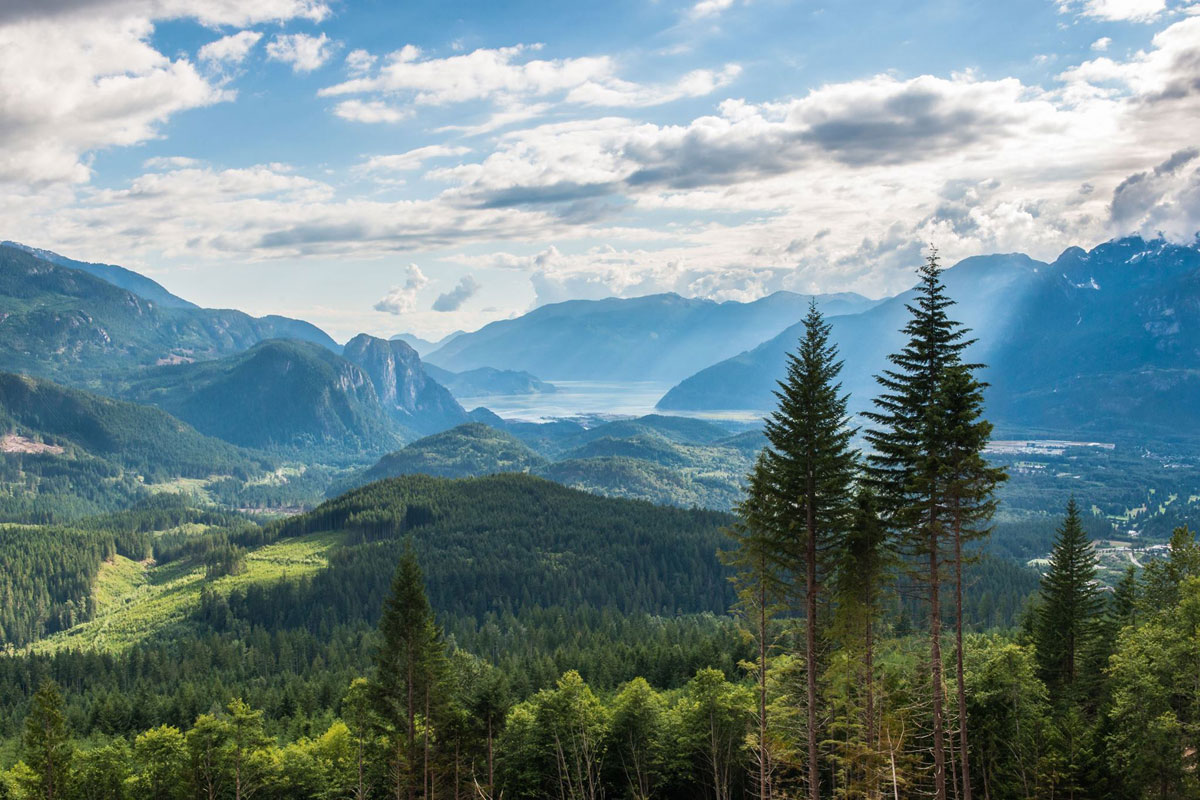
British Columbia is home to one of our most important natural resources: forests; however, monitoring them used to be a labor-intensive activity. Luckily, remote sensing techniques are becoming the mainstream solution. Today, I will blog about one method we can leverage, Lidar (Light Detection and Ranging), to automate some work and help sustain our green planet. I will also walk through how I use lidR (an R package developed for forestry applications) to “visit” Saint Joe National Forest. Why not somewhere in BC? Because I could not find the relevant data on OpenTopography.

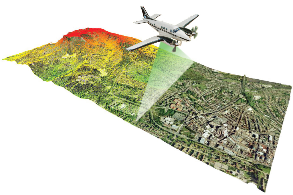
Lidar can be collected by small aircraft. The laser device sends pulses of light to the ground surface and waits for it to reflect, whose travel time can be used to determine the distance to various objects. It is not uncommon to fly a drone to collect Lidar. As you can probably imagine, the data (point cloud) can play an essential role in city planning, archaeology, and climate monitoring. The scaling effect is enormous in forestry if we can measure the canopy heights or thickness without physically going there.

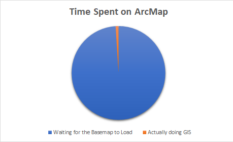
There is commercial and open-source software, such as ArcGIS and QGIS, specialized in advanced processing and analyzing the data. Initially, I bought the personal use ArcGIS license but found that it requires Windows to run. I will do another blog post when I figure out how to use it. But for now, as a data scientist, I have decided to use lidR for some experiments. I find that it is sufficient to process a smaller region of data on my Mac (16GB RAM).

There are many sites to get open-sourced lidar data, and one of the most popular ones is OpenTopography. You can view the data map and zoom in to any region with the dot. It lets you download the unclassified point cloud in either compressed (LAZ) or uncompressed (LAS) format, with optional adds on such as Digital Terrain Models (DTM). I downloaded a LAZ file containing a small area in the St. Joe National Forest with 169 thousand points for learning purposes.

Vegetation analysis using lidR

Next, I will show you standard processing for the point cloud and vegetation analysis using lidR. Btw, lidR on GitHub is an excellent handbook to follow.

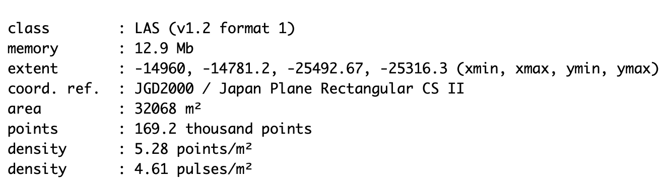
First, let’s read the LAZ format into the R object using the following command. When we print the object, it shows some metadata, such as the number of points, the measuring unit in meters, and the coordination reference.

las <- readLAS("/Users/elaineye/Desktop/lidar/forest_points.laz")
print(las)

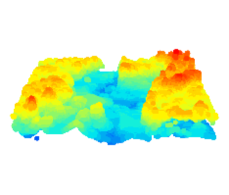
Like any other data analysis, we must do some pre-processing steps. We will generate what the earth is like in the so-called Digital Terrain Model (DTM). The idea is to interpolate the known ground points to produce a continuous surface. I used the built-in Invert distance weighting (IDW) algorithm, which takes the weighted average of neighboring points to approximate the unknown. The terrain is plotted below.

dtm_idw <- rasterize_terrain(las, algorithm = knnidw())
plot_dtm3d(dtm_idw, bg = "white") 

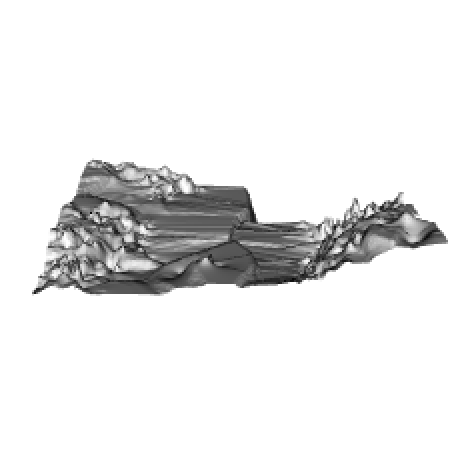
Wait, the surface looks uneven, and it is impossible to produce any meaningful metrics if the elevation is not relative to the ground. Hence we need to do some height normalization by subtracting the LAS from the DTM. Now the plot looks right.

nlas <- las - dtm_idw
plot(nlas, size=4, bg="white")

Since our end goal is to calculate tree-level metrics, we must first segment trees. lidR package provides a point-to-raster algorithm that produces the canopy height model (CHM) used for tree top detection. Here we define the pixel value as 0.5 m, meaning each pixel represents the highest elevation of a 0.5 m by 0.5 m square.

# Point-to-raster 2 resolutions
chm_p2r_05 <- rasterize_canopy(nlas, 0.5, p2r())

We then apply a medium filter with some post-processing steps to remove noise created by local irregularities of branches. How the local maxima filter works is beyond the scope of this post, but there are lots of resources that explain it.

kernel <- matrix(1,3,3)
chm_p2r_05_smoothed <- terra::focal(chm_p2r_05, w = kernel, fun = median, na.rm = TRUE)
ttops_chm_p2r_05_smoothed <- locate_trees(chm_p2r_05_smoothed, lmf(5))

algo <- dalponte2016(chm_p2r_05_smoothed, ttops_chm_p2r_05_smoothed)

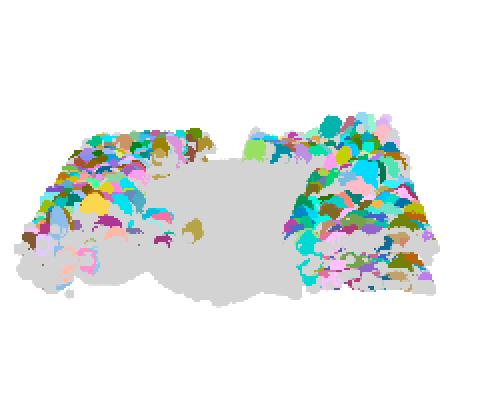
We can now run the segment_trees method on the DTM with the above algorithm and see the colorful trees!

nlas <- segment_trees(nlas, algo) 
plot(nlas, bg = "white", size = 4, color = "treeID") 

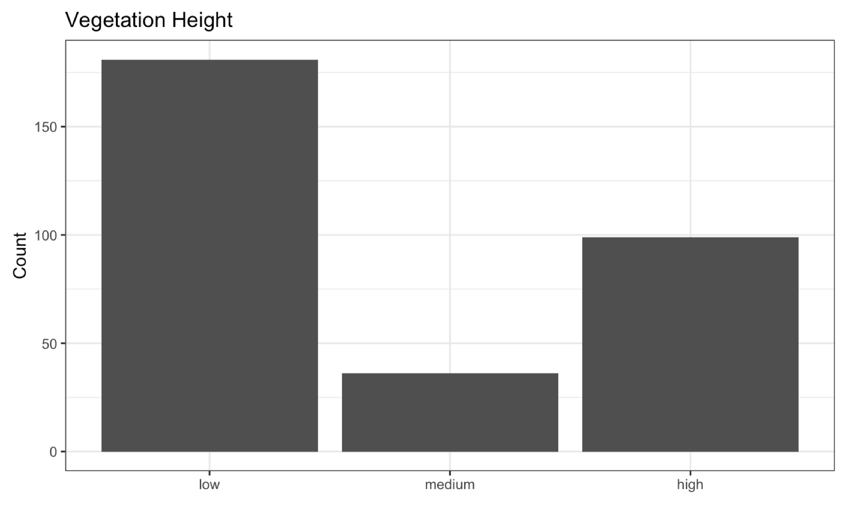
Lastly, we will classify the vegetation based on its heights. According to the Ministry of Environment, trees are classified as low (over 1.5 m and under 6 m), medium (over 6 m and under 10m), and high if they are greater than 10 m. We can calculate the crown metrics given any custom functions, in this case, max.

metrics <- crown_metrics(nlas, ~list(z_max = max(Z)))

I will conclude the activity with a histogram showing the number of different vegetation types.

I hope this post blog gives you an idea of lidar and some basic processing in the lidR package in the context of forestry applications. I am new to GIS, but I have found it fascinating. With more data and advanced tooling, we will better understand our planet, and a sustainable environment will become possible.